Real world Pandas: Cut and Where
Mon 08 April 2013
I forgot to mention in the last post why this series is called Real World Pandas. The Pandas documentation is really, really great, and the examples are exactly what I would want starting out- simple foo/bar/baz type of tables that make it simple to see what transformations are happening. The goal of these blog posts is to show a few examples of "real-world" applications, similar to Wes McKinney's examples in his book. A book I highly recommend, btw- not only is the Pandas stuff great, as you would expect, but it has one of the best Python crash courses I've read, as well a great intro to IPython, Numpy, and Matplotlib. I still find myself referencing it.
Lets again pull in some data from my examples folder in the climatic repo.
import pandas as pd
import numpy as np
import climatic as cl

walsenburg = cl.MetMast()
walsenburg.wind_import(r'CO_Walsenburg_South_Data.txt',
                       header_row=0, time_col=0,
                       delimiter='\t', smart_headers=True)
Now let's generate a weibull distribution:
walsenburg.weibull(['WS Mean 1', 50.0])
This will generate both binned data and a continuous distribution of the WS Mean 1 signal: 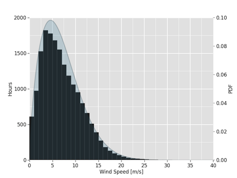
Going behind the scenes again:
>>>import numpy as np

#Grab wind speed column
>>>ws_data = walsenburg.data[('WS Mean 1', 50.0)]

#Build your range, use pd.cut to bin the data
>>>ws_range = np.arange(0, ws_data.max() + 1, 1)
>>>binned = pd.cut(ws_data, ws_range)

#Do a simple value counts to get your histogram, then reindex to
#align the bins from 0-31:
>>>dist_10min = pd.value_counts(binned).reindex(binned.levels)
(0, 1]       3650
(1, 2]       5813
(2, 3]       9139
(3, 4]      10917
(4, 5]      10648
(5, 6]      10072
(6, 7]       9302
(7, 8]       8020
(8, 9]       7105
(9, 10]      6351
(10, 11]     5703
(11, 12]     4783
(12, 13]     3954
(13, 14]     3058
(14, 15]     2318
(15, 16]     1614
(16, 17]     1074
(17, 18]      780
(18, 19]      544
(19, 20]      403
(20, 21]      274
(21, 22]      186
(22, 23]      133
(23, 24]       99
(24, 25]       75
(25, 26]       59
(26, 27]       27
(27, 28]       23
(28, 29]        9
(29, 30]        5
(30, 31]        2

#Counts are good, but I want to add a couple more columns. Lets
#turn the series into a dataframe:
>>>dist = pd.DataFrame({'Binned: 10Min': dist_10min})

#Now lets get the number of hours in each bin, and some
#normalized values:
>>>dist['Binned: Hourly'] = dist['Binned: 10Min']/6
>>>dist.fillna(0) #No data, zero hours...
>>>dist['Normed'] = (dist['Binned: 10Min']/dist['Binned: 10Min'].sum())*100
>>>dist
          Binned: 10Min  Binned: Hourly     Normed
(0, 1]             3650      608.333333   3.438854
(1, 2]             5813      968.833333   5.476729
(2, 3]             9139     1523.166667   8.610326
(3, 4]            10917     1819.500000  10.285472
(4, 5]            10648     1774.666667  10.032033
(5, 6]            10072     1678.666667   9.489354
(6, 7]             9302     1550.333333   8.763897
(7, 8]             8020     1336.666667   7.556058
(8, 9]             7105     1184.166667   6.693989
(9, 10]            6351     1058.500000   5.983607
(10, 11]           5703      950.500000   5.373092
(11, 12]           4783      797.166667   4.506312
(12, 13]           3954      659.000000   3.725269
(13, 14]           3058      509.666667   2.881100
(14, 15]           2318      386.333333   2.183908
(15, 16]           1614      269.000000   1.520633
(16, 17]           1074      179.000000   1.011871
(17, 18]            780      130.000000   0.734878
(18, 19]            544       90.666667   0.512531
(19, 20]            403       67.166667   0.379687
(20, 21]            274       45.666667   0.258150
(21, 22]            186       31.000000   0.175240
(22, 23]            133       22.166667   0.125306
(23, 24]             99       16.500000   0.093273
(24, 25]             75       12.500000   0.070661
(25, 26]             59        9.833333   0.055587
(26, 27]             27        4.500000   0.025438
(27, 28]             23        3.833333   0.021669
(28, 29]              9        1.500000   0.008479
(29, 30]              5        0.833333   0.004711
(30, 31]              2        0.333333   0.001884
In just a few lines of Pandas, we went from a pile of data to nicely binned data.
One more quick example for this week: using the .where method on a dataframe to filter for the data you want. When analyzing wind data, its very common to have a "Flag" column that indicates whether or not a datapoint should be filtered. Let's concat a new small example dataframe and make up some flags:
>>>data = pd.concat([walsenburg.data['WS Mean 1', 50.0][:20],
                     walsenburg.data[('WS Mean 2', 50.0)][:20]], axis=1)
>>>data['Flag'] = [random.randint(0, 1) for x in range(0, 20, 1)]
>>>data

                     (WS Mean 1, 50.0)  (WS Mean 2, 50.0)  Flag
Date & Time Stamp
2010-06-01 14:00:00              12.05              12.26     1
2010-06-01 14:10:00              11.48              11.60     1
2010-06-01 14:20:00              14.19              14.39     1
2010-06-01 14:30:00              13.21              13.43     0
2010-06-01 14:40:00              11.92              12.12     0
2010-06-01 14:50:00              11.90              12.05     1
2010-06-01 15:00:00              12.78              12.92     0
2010-06-01 15:10:00              13.27              13.40     1
2010-06-01 15:20:00              14.05              14.24     1
2010-06-01 15:30:00              13.32              13.48     1
2010-06-01 15:40:00              15.32              15.43     1
2010-06-01 15:50:00              16.60              16.70     0
2010-06-01 16:00:00              15.91              16.01     1
2010-06-01 16:10:00              15.62              15.73     1
2010-06-01 16:20:00              15.16              15.24     1
2010-06-01 16:30:00              15.96              16.06     0
2010-06-01 16:40:00              14.84              15.02     0
2010-06-01 16:50:00              15.14              15.30     1
2010-06-01 17:00:00              14.33              14.49     0
2010-06-01 17:10:00              13.20              13.37     1
Now I want a create a new wind speed column with only rows where Flag == 0:
>>>data['Flag WS 1'] = data[('WS Mean 1', 50.0)].where(data['Flag'] == 0)
>>>data

                     (WS Mean 1, 50.0)  (WS Mean 2, 50.0)  Flag  Flag WS 1
Date & Time Stamp
2010-06-01 14:00:00              12.05              12.26     1        NaN
2010-06-01 14:10:00              11.48              11.60     1        NaN
2010-06-01 14:20:00              14.19              14.39     1        NaN
2010-06-01 14:30:00              13.21              13.43     0      13.21
2010-06-01 14:40:00              11.92              12.12     0      11.92
2010-06-01 14:50:00              11.90              12.05     1        NaN
2010-06-01 15:00:00              12.78              12.92     0      12.78
2010-06-01 15:10:00              13.27              13.40     1        NaN
2010-06-01 15:20:00              14.05              14.24     1        NaN
2010-06-01 15:30:00              13.32              13.48     1        NaN
2010-06-01 15:40:00              15.32              15.43     1        NaN
2010-06-01 15:50:00              16.60              16.70     0      16.60
2010-06-01 16:00:00              15.91              16.01     1        NaN
2010-06-01 16:10:00              15.62              15.73     1        NaN
2010-06-01 16:20:00              15.16              15.24     1        NaN
2010-06-01 16:30:00              15.96              16.06     0      15.96
2010-06-01 16:40:00              14.84              15.02     0      14.84
2010-06-01 16:50:00              15.14              15.30     1        NaN
2010-06-01 17:00:00              14.33              14.49     0      14.33
2010-06-01 17:10:00              13.20              13.37     1        NaN
I also could have replaced any flagged value with another value:
>>>data['Flag WS 1'] = data[('WS Mean 1', 50.0)].where(data['Flag'] == 0, -999)

                     (WS Mean 1, 50.0)  (WS Mean 2, 50.0)  Flag  Flag WS 1
Date & Time Stamp
2010-06-01 14:00:00              12.05              12.26     1    -999.00
2010-06-01 14:10:00              11.48              11.60     1    -999.00
2010-06-01 14:20:00              14.19              14.39     1    -999.00
2010-06-01 14:30:00              13.21              13.43     0      13.21
2010-06-01 14:40:00              11.92              12.12     0      11.92
2010-06-01 14:50:00              11.90              12.05     1    -999.00
2010-06-01 15:00:00              12.78              12.92     0      12.78
2010-06-01 15:10:00              13.27              13.40     1    -999.00
2010-06-01 15:20:00              14.05              14.24     1    -999.00
2010-06-01 15:30:00              13.32              13.48     1    -999.00
2010-06-01 15:40:00              15.32              15.43     1    -999.00
2010-06-01 15:50:00              16.60              16.70     0      16.60
2010-06-01 16:00:00              15.91              16.01     1    -999.00
2010-06-01 16:10:00              15.62              15.73     1    -999.00
2010-06-01 16:20:00              15.16              15.24     1    -999.00
2010-06-01 16:30:00              15.96              16.06     0      15.96
2010-06-01 16:40:00              14.84              15.02     0      14.84
2010-06-01 16:50:00              15.14              15.30     1    -999.00
2010-06-01 17:00:00              14.33              14.49     0      14.33
2010-06-01 17:10:00              13.20              13.37     1    -999.00
Next week I hope to cover some ways to manipulate a MultiIndex and Panels to group data in logical and helpful ways. Thanks for reading!