Mapping Data in Python with Pandas and Vincent
Tue 08 October 2013
One area where the Pandas/Vincent workflow really shines is in Data Exploration- rapidly iterating DataFrames with Vincent visualizations to explore your data and find the best visual representation. With the release of Vincent 0.3, you can now also rapidly iterate maps to visualize your data.
Disclaimer: there are certainly still some deficiencies in Vega.js that make building production-quality maps tough. The tools to perform more detailed projection manipulations are still lacking (though it wouldnt take much work to the right pipes hooked up). For high quality map publishing, I still recommend using raw D3. However, for very quick exploration with Python data, it's tough to beat Vincent/Vega.
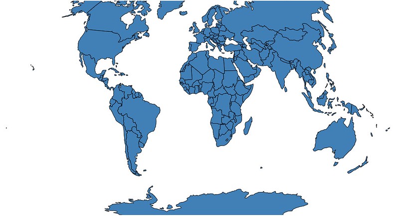
Let's start with a very simple map of the world to show how to add a map chart in Vincent. All of the geodata here can be found in the vincent_map_data repo.
A simple map of the world:
import vincent
geo_data = [{'name': 'countries',
             'url': world_topo,
             'feature': 'world-countries'}]

vis = vincent.Map(geo_data=geo_data, scale=200)
vis.to_json('vega.json')
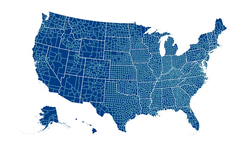
Vincent also allows for passing multiple map layers:
geo_data = [{'name': 'counties',
             'url': county_topo,
             'feature': 'us_counties.geo'},
            {'name': 'states',
             'url': state_topo,
             'feature': 'us_states.geo'}
             ]

vis = vincent.Map(geo_data=geo_data, scale=1000, projection='albersUsa')
#Get rid of State fill, customize stroke color
del vis.marks[1].properties.update
vis.marks[0].properties.update.fill.value = '#084081'
vis.marks[1].properties.enter.stroke.value = '#fff'
vis.marks[0].properties.enter.stroke.value = '#7bccc4'
Now to the data exploration: mapping data in Pandas DataFrames to TopoJSON to create a choropleth visualization. First, some mild data munging to ensure that your data will key correctly with the TopoJSON properties:
import json
import pandas as pd
#Map the county codes we have in our geometry to those in the
#county_data file, which contains additional rows we don't need
with open('us_counties.topo.json', 'r') as f:
    get_id = json.load(f)

#A little FIPS code type casting to ensure keys match
new_geoms = []
for geom in get_id['objects']['us_counties.geo']['geometries']:
    geom['properties']['FIPS'] = int(geom['properties']['FIPS'])
    new_geoms.append(geom)

get_id['objects']['us_counties.geo']['geometries'] = new_geoms

with open('us_counties.topo.json', 'w') as f:
    json.dump(get_id, f)

#Grab the FIPS codes and load them into a dataframe
geometries = get_id['objects']['us_counties.geo']['geometries']
county_codes = [x['properties']['FIPS'] for x in geometries]
county_df = pd.DataFrame({'FIPS': county_codes}, dtype=str)
county_df = county_df.astype(int)

#Read county unemployment data into Dataframe, cast to int for consistency
df = pd.read_csv('data/us_county_data.csv', na_values=[' '])
df['FIPS'] = df['FIPS'].astype(int)

#Perform an inner join, pad NA's with data from nearest county
merged = pd.merge(df, county_df, on='FIPS', how='inner')
merged = merged.fillna(method='pad')
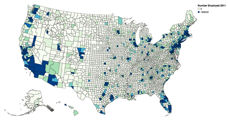
Now we can set up our map:
geo_data = [{'name': 'counties',
             'url': county_topo,
             'feature': 'us_counties.geo'}]

vis = vincent.Map(data=merged, geo_data=geo_data, scale=1100,
                  projection='albersUsa', data_bind='Employed_2011',
                  data_key='FIPS', map_key={'counties': 'properties.FIPS'})
vis.marks[0].properties.enter.stroke_opacity = ValueRef(value=0.5)
#Change our domain for an even inteager
vis.scales['color'].domain = [0, 189000]
vis.legend(title='Number Employed 2011')
vis.to_json('vega.json')
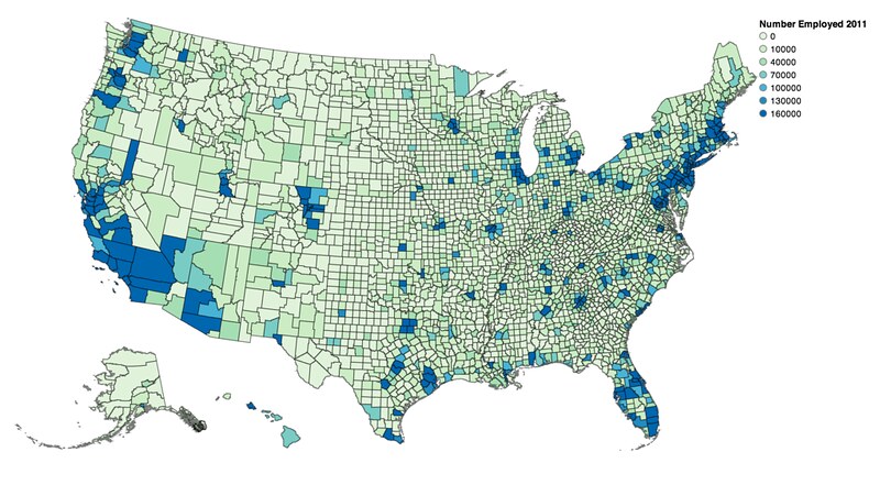
Vincent defaults your scale to a quantize scale between [0, column.quantile(0.95)], but custom scales are encouraged:
vis.scales['color'].type = 'threshold'
vis.scales['color'].domain = [0, 10000, 40000, 70000, 100000, 130000, 160000]
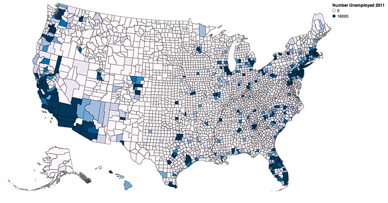
Data can be quickly rebound with new columns and new color brewer scales to rapidly visualize different columns of the DataFrame:
vis.rebind(column='Unemployed_2011', brew='PuBu')
vis.scales['color'].domain = [0, 18000]
vis.legends[0].title = 'Number Unemployed 2011'
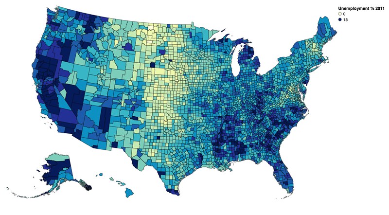
vis.rebind(column='Unemployment_rate_2011', brew='YlGnBu')
vis.scales['color'].domain = [0, 15]
vis.legends[0].title = 'Unemployment % 2011'
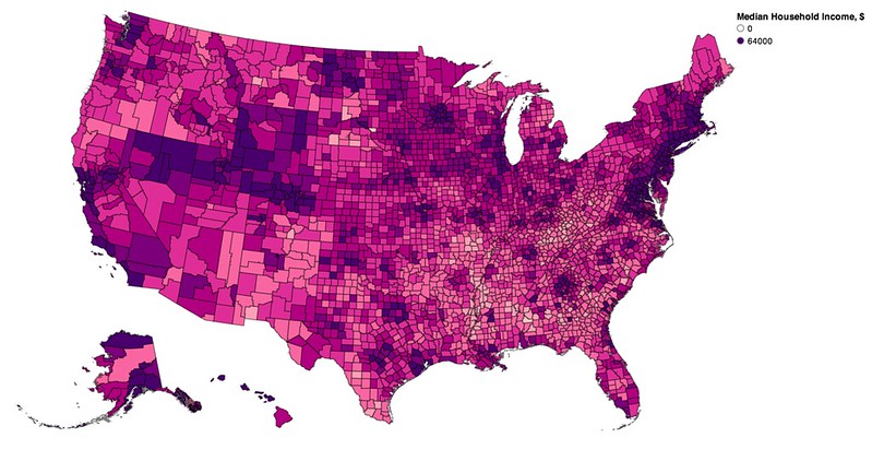
vis.rebind(column='Median_Household_Income_2011', brew='RdPu')
vis.scales['color'].domain = [0, 64000]
vis.legends[0].title = 'Median Household Income, $'
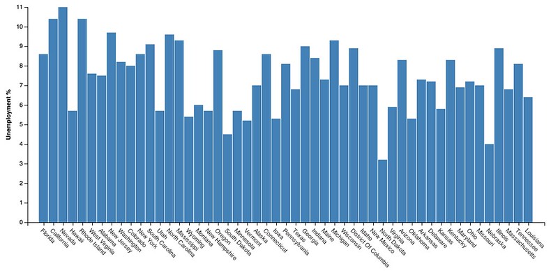
Let's run through a quick example at the state level, looking at a bar chart first:
yoy = pd.read_table('data/State_Unemp_YoY.txt', delim_whitespace=True)
#Standardize State names to match TopoJSON for keying
vis = vincent.Bar(yoy, columns=['AUG_2012'], key_on='NAME', height=400)
vis.axes[0].properties = AxisProperties(
    labels=PropertySet(
        angle=ValueRef(value=45),
        align=ValueRef(value='left')
        )
    )
vis.padding['bottom'] = 90
vis.axis_titles(y='Unemployment %', x='')
vis.to_json('vega.json')
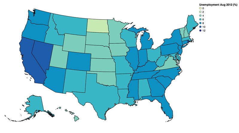
Now we can look at the geo:
#Make sure names match TopoJSON
names = []
for row in yoy.iterrows():
    pieces = row[1]['NAME'].split('_')
    together = ' '.join(pieces)
    names.append(together.title())
yoy['NAME'] = names

geo_data = [{'name': 'states',
             'url': state_topo,
             'feature': 'us_states.geo'}]
vis = vincent.Map(data=yoy, geo_data=geo_data, scale=1000,
                  projection='albersUsa', data_bind='AUG_2012', data_key='NAME',
                  map_key={'states': 'properties.NAME'}, brew='YlGnBu')
#Custom threshold scale
vis.scales[0].type='threshold'
vis.scales[0].domain = [0, 2, 4, 6, 8, 10, 12]
vis.legend(title='Unemployment Aug 2012 (%)')
vis.to_json('vega.json')
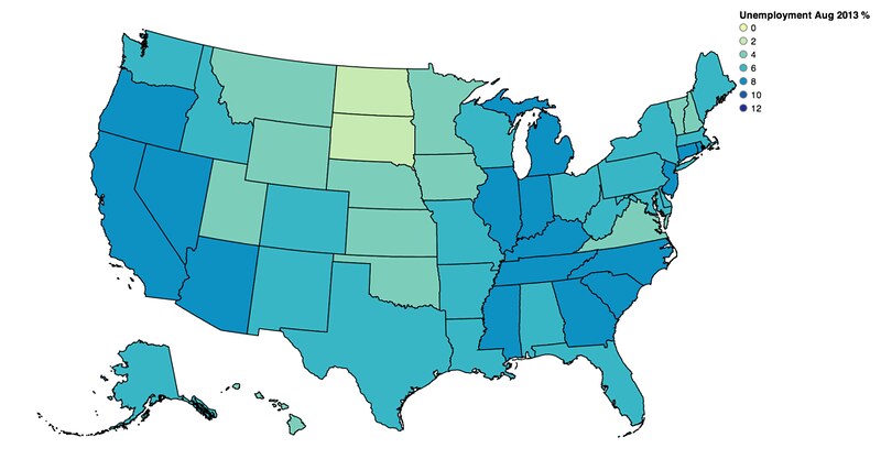
Rebind and revisualize:
vis.rebind(column='AUG_2013', brew='YlGnBu')
vis.scales[0].type='threshold'
vis.scales[0].domain = [0, 2, 4, 6, 8, 10, 12]
vis.legends[0].title = 'Unemployment Aug 2013 %'
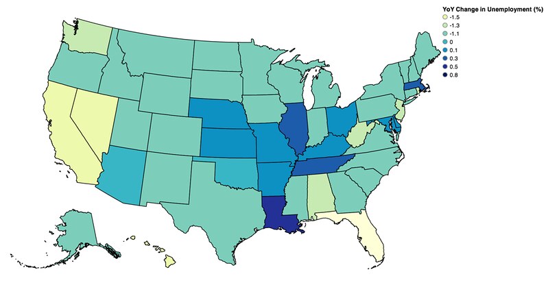
Finally, the % change Year over Year:
vis.rebind(column='CHANGE', brew='YlGnBu')
vis.scales[0].type='threshold'
vis.scales[0].domain = [-1.5, -1.3, -1.1, 0, 0.1, 0.3, 0.5, 0.8]
vis.legends[0].title = "YoY Change in Unemployment (%)"
One more example, this one showing where Vega falls a bit short at the moment. This was about the best I could do to map Oregon county populations:
#Oregon County-level population data
or_data = pd.read_table('data/OR_County_Data.txt', delim_whitespace=True)
or_data['July_2012_Pop']= or_data['July_2012_Pop'].astype(int)
#Standardize keys
with open('or_counties.topo.json', 'r') as f:
    counties = json.load(f)

def split_county(name):
    parts = name.split(' ')
    parts.pop(-1)
    return ''.join(parts).upper()

#A little FIPS code munging
new_geoms = []
for geom in counties['objects']['or_counties.geo']['geometries']:
    geom['properties']['COUNTY'] = split_county(geom['properties']['COUNTY'])
    new_geoms.append(geom)

counties['objects']['or_counties.geo']['geometries'] = new_geoms

with open('or_counties.topo.json', 'w') as f:
    json.dump(counties, f)

geo_data = [{'name': 'states',
             'url': state_topo,
             'feature': 'us_states.geo'},
            {'name': 'or_counties',
             'url': or_topo,
             'feature': 'or_counties.geo'}]

vis = vincent.Map(data=or_data, geo_data=geo_data, scale=3700,
                  translate=[1480, 830], projection='albersUsa',
                  data_bind='July_2012_Pop', data_key='NAME',
                  map_key={'or_counties': 'properties.COUNTY'})
vis.marks[0].properties.update.fill.value = '#c2c2c2'
vis.to_json('vega.json')
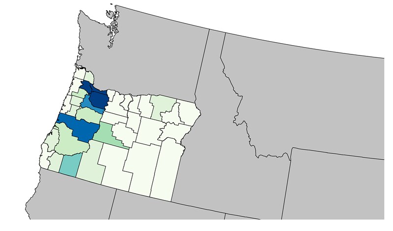
Of course, albersUsa isn't the right projection to just get the state- we really probably want something like conicConformal. Also, to properly center correctly, Vega needs to take D3.geo parameters such as parallels and a rotation array (right now it takes a single number).
So- once you've got your data in the right format, and your geodata properly TopoJSONized, Vincent + Pandas can allow for rapid iteration of geo visualizations. Happy mapmaking!