Real world Pandas: Indexing and Plotting with the MultiIndex
Wed 17 April 2013
The MultiIndex is one of the most valuable tools in the Pandas library, particularly if you are working with data that's heavy on columns and attributes. I was going to tackle Panels as well this time (as they can complement MultiIndexing in many ways), but the next version on Pandas that is on the cusp of release is about to introduce some new indexing tools that should make accessing minor and major axes in Panels better than before. Stay tuned.
Again using my data from the examples folder in the climatic repo.
import pandas as pd
import numpy as np
import climatic as cl

walsenburg = cl.MetMast()
walsenburg.wind_import(r'CO_Walsenburg_South_Data.txt',
                       header_row=0, time_col=0,
                       delimiter='\t', smart_headers=True)
Our dataframe is a little...busy:
>>>df = walsenburg.data
>>>df
<class pandas.core.frame.DataFrame'>
DatetimeIndex: 106140 entries, 2010-06-01 14:00:00 to 2012-06-07 15:50:00
Data columns:
(WS Mean 1, 50.0)      106140  non-null values
(WS StdDev 1, 50.0)    106140  non-null values
(WS Max 1, 50.0)       106140  non-null values
(WS Min 1, 50.0)       106140  non-null values
(WS Mean 2, 50.0)      106140  non-null values
(WS StdDev 2, 50.0)    106140  non-null values
(WS Max 2, 50.0)       106140  non-null values
(WS Min 2, 50.0)       106140  non-null values
(WS Mean 3, 30.0)      106140  non-null values
(WS StdDev 3, 30.0)    106140  non-null values
(WS Max 3, 30.0)       106140  non-null values
(WS Min 3, 30.0)       106140  non-null values
(WS Mean 4, 40.0)      106140  non-null values
(WS StdDev 4, 40.0)    106140  non-null values
(WS Max 4, 40.0)       106140  non-null values
(WS Min 4, 40.0)       106140  non-null values
(WD Mean 1, 49.0)      106140  non-null values
(WD StdDev 1, 49.0)    106140  non-null values
(WD Max 1, 49.0)       106140  non-null values
(WD Min 1, 49.0)       106140  non-null values
(WD Mean 2, 38.0)      106140  non-null values
(WD StdDev 2, 38.0)    106140  non-null values
(WD Max 2, 38.0)       106140  non-null values
(WD Min 2, 38.0)       106140  non-null values
dtypes: float64(16), int64(8)
It would be really useful to be able to index the signals for each height. Since our columns are already tuples, Pandas lets us create a MultiIndex in one line and then apply it to our dataframe:
>>>multi_cols = pd.MultiIndex.from_tuples(df, names=['Signals', 'Heights'])
>>>df.columns = multi_cols
>>>df.columns
MultiIndex
[(WS Mean 1, 50.0), (WS StdDev 1, 50.0), (WS Max 1, 50.0), (WS Min 1, 50.0),
 (WS Mean 2, 50.0), (WS StdDev 2, 50.0), (WS Max 2, 50.0), (WS Min 2, 50.0),
 (WS Mean 3, 30.0), (WS StdDev 3, 30.0), (WS Max 3, 30.0), (WS Min 3, 30.0),
 (WS Mean 4, 40.0), (WS StdDev 4, 40.0), (WS Max 4, 40.0), (WS Min 4, 40.0),
 (WD Mean 1, 49.0), (WD StdDev 1, 49.0), (WD Max 1, 49.0), (WD Min 1, 49.0),
 (WD Mean 2, 38.0), (WD StdDev 2, 38.0), (WD Max 2, 38.0), (WD Min 2, 38.0)]
Those columns still look busy- except now we can index by signal:
>>>df['WS Mean 1'].head()
                        50
Date & Time Stamp
2010-06-01 14:00:00  12.05
2010-06-01 14:10:00  11.48
2010-06-01 14:20:00  14.19
2010-06-01 14:30:00  13.21
2010-06-01 14:40:00  11.92
Nice! This is a little more useful, but it would be more helpful if our unique signals weren't at the top level, since the signals are grouped by height, rather than vice versa. Let's do a swap (this is why we named our levels in the previous step):
>>>df = df.swaplevel('Signals', 'Heights', axis=1)
Now we can conveniently index by height:
>>>df[50.0]
<class pandas.core.frame.DataFrame'>
DatetimeIndex: 106140 entries, 2010-06-01 14:00:00 to 2012-06-07 15:50:00
Data columns:
WS Mean 1      106140  non-null values
WS StdDev 1    106140  non-null values
WS Max 1       106140  non-null values
WS Min 1       106140  non-null values
WS Mean 2      106140  non-null values
WS StdDev 2    106140  non-null values
WS Max 2       106140  non-null values
WS Min 2       106140  non-null values
dtypes: float64(8)
This is a lot more useful than having tuples for all of the columns.
The wind shear is a pretty common thing to calculate when doing wind data analysis, and for that calc we really just want mean wind speeds for each height. One option is to loop through the columns of our original dataframe and pull out the ones we need, then put the pieces back together with pd.concat:
>>>df = walsenburg.data #Back to our original dataframe
>>>series_list = []
>>>for col in df.iterkv():
       if 'WS Mean' in col[0][0]:
           #Create array levels so that the dataframe will build a MultiIndex
           levels = [np.array([col[0][1]]), np.array([col[0][0]])]
           temp_df = pd.DataFrame(col[1], columns=levels)
           series_list.append(temp_df)
>>>df2 = pd.concat(series_list, axis=1) #Put the pieces together
>>>df2.head()
                            50                    30         40
                     WS Mean 1  WS Mean 2  WS Mean 3  WS Mean 4
Date & Time Stamp
2010-06-01 14:00:00      12.05      12.26      11.38      11.70
2010-06-01 14:10:00      11.48      11.60      10.76      11.14
2010-06-01 14:20:00      14.19      14.39      13.35      13.84
2010-06-01 14:30:00      13.21      13.43      12.43      12.94
2010-06-01 14:40:00      11.92      12.12      11.32      11.60
Very nice! What if wanted to look at all of the signals, with column levels for height, signal (WS, WD, etc), and signal attribute (Mean, Max, etc)? Just a small tweak:
>>>series_list = []
>>>for col in df.iterkv():
       splitter = col[0][0].split()
       signal = splitter[0]
       att = ' '.join([splitter[1], splitter[2]])
       height = col[0][1]
       levels = [np.array([height]), np.array([signal]), np.array([att])]
       temp_df = pd.DataFrame(col[1], columns=levels)
       series_list.append(temp_df)
>>>df3 = pd.concat(series_list, axis=1) #Put the pieces together
Now we can index with multiple keys to both height and signal:
>>>df3[50]['WS'][0:10]
                         Mean 1  StdDev 1  Max 1  Min 1  Mean 2  StdDev 2  Max 2  Min 2
Date & Time Stamp
2010-06-01 14:00:00      12.05      2.14  15.90   7.91   12.26      2.25  16.30   7.94
2010-06-01 14:10:00      11.48      2.24  17.40   6.40   11.60      2.35  17.47   6.04
2010-06-01 14:20:00      14.19      2.24  19.30   9.06   14.39      2.35  19.37   9.09
2010-06-01 14:30:00      13.21      1.58  17.40   9.82   13.43      1.66  17.84   9.48
2010-06-01 14:40:00      11.92      1.73  15.48   7.53   12.12      1.89  15.96   7.56
2010-06-01 14:50:00      11.90      1.73  16.24   7.53   12.05      1.81  16.30   7.56
2010-06-01 15:00:00      12.78      1.45  16.63   9.06   12.92      1.46  16.70   8.72
2010-06-01 15:10:00      13.27      1.65  18.15   9.44   13.40      1.73  18.22   9.48
2010-06-01 15:20:00      14.05      1.80  18.15   9.82   14.24      1.81  18.62   9.86
2010-06-01 15:30:00      13.32      1.80  19.66   9.06   13.48      1.81  19.74   9.09

>>>df3[49]['WD'].tail()
                     Mean 1  StdDev 1  Max 1  Min 1
Date & Time Stamp
2012-06-07 15:10:00      86        33     80    240
2012-06-07 15:20:00     228        24    231    240
2012-06-07 15:30:00     224        16    210    240
2012-06-07 15:40:00     234        13    233    240
2012-06-07 15:50:00     238        13    234    240
We sorted levels earlier using level names- you can actually use integer indexing as well. Lets sort for signals at the top, then height, then attributes:
>>>df3.reorder_levels([1, 0, 2], axis=1)
<class pandas.core.frame.DataFrame'>
DatetimeIndex: 106140 entries, 2010-06-01 14:00:00 to 2012-06-07 15:50:00
Data columns:
(WS, 50.0, Mean 1)      106140  non-null values
(WS, 50.0, StdDev 1)    106140  non-null values
(WS, 50.0, Max 1)       106140  non-null values
(WS, 50.0, Min 1)       106140  non-null values
(WS, 50.0, Mean 2)      106140  non-null values
(WS, 50.0, StdDev 2)    106140  non-null values
(WS, 50.0, Max 2)       106140  non-null values
(WS, 50.0, Min 2)       106140  non-null values
(WS, 30.0, Mean 3)      106140  non-null values
(WS, 30.0, StdDev 3)    106140  non-null values
(WS, 30.0, Max 3)       106140  non-null values
(WS, 30.0, Min 3)       106140  non-null values
(WS, 40.0, Mean 4)      106140  non-null values
(WS, 40.0, StdDev 4)    106140  non-null values
(WS, 40.0, Max 4)       106140  non-null values
(WS, 40.0, Min 4)       106140  non-null values
(WD, 49.0, Mean 1)      106140  non-null values
(WD, 49.0, StdDev 1)    106140  non-null values
(WD, 49.0, Max 1)       106140  non-null values
(WD, 49.0, Min 1)       106140  non-null values
(WD, 38.0, Mean 2)      106140  non-null values
(WD, 38.0, StdDev 2)    106140  non-null values
(WD, 38.0, Max 2)       106140  non-null values
(WD, 38.0, Min 2)       106140  non-null values
dtypes: float64(16), int64(8)
If you are using tuples for your column or row names, I highly recommend building a MultiIndex out of them, as it allows for you to index and manipulate data very efficiently.
One last thing: I wrote a little library called Vincent to plot data using Vega. Lets look at WS 1 vs WS 4 for the first ten days of data, passing our new MultiIndex to Vincent:
>>>data = df3['2010-06-01':'2010-06-11']
>>>import vincent
>>>vis = vincent.Scatter()
#Pass the levels as tuples
>>>vis.tabular_data(data, columns=[(50, 'WS', 'Mean 1'), (40, 'WS', 'Mean 4')])
>>>vis.to_json(r'/vega.json', split_data=True, html=True)
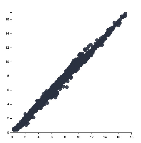
It's a little...bloated, for lack of a better word. Let's remove fill and make the marks smaller:
>>>vis + ('transparent', 'marks', 0, 'properties', 'update', 'fill', 'value')
>>>vis + ({'value': 25}, 'marks', 0, 'properties', 'update', 'size')
>>>vis.to_json(r'/vega.json', split_data=True, html=True)
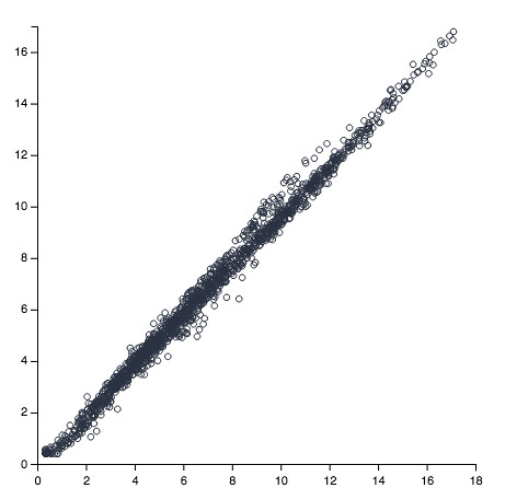
Better. Still need some axis labels, which is something I need to figure out how to do within Vega and make easy in Python. As always, thanks for reading!